POVM

In functional analysis and quantum information science, a positive operator-valued measure (POVM) is a measure whose values are positive semi-definite operators on a Hilbert space. POVMs are a generalization of projection-valued measures (PVM) and, correspondingly, quantum measurements described by POVMs are a generalization of quantum measurement described by PVMs (called projective measurements).

In rough analogy, a POVM is to a PVM what a mixed state is to a pure state. Mixed states are needed to specify the state of a subsystem of a larger system (see purification of quantum state); analogously, POVMs are necessary to describe the effect on a subsystem of a projective measurement performed on a larger system.

POVMs are the most general kind of measurement in quantum mechanics, and can also be used in quantum field theory.^[1] They are extensively used in the field of quantum information.

Definition

Let ${\displaystyle {\mathcal {H}}}$ denote a Hilbert space and ${\displaystyle (X,M)}$ a measurable space with ${\displaystyle M}$ a Borel σ-algebra on ${\displaystyle X}$. A POVM is a function ${\displaystyle F}$ defined on ${\displaystyle M}$ whose values are positive bounded self-adjoint operators on ${\displaystyle {\mathcal {H}}}$ such that for every ${\displaystyle \psi \in {\mathcal {H}}}$

${\displaystyle E\mapsto \langle F(E)\psi \mid \psi \rangle ,}$

is a non-negative countably additive measure on the σ-algebra ${\displaystyle M}$ and ${\displaystyle F(X)=\operatorname {I} _{\mathcal {H}}}$ is the identity operator.^[2]

In the simplest case, a POVM is a set of positive semi-definite Hermitian matrices ${\displaystyle \{F_{i}\}}$ on a finite-dimensional Hilbert space ${\displaystyle {\mathcal {H}}}$ that sum to the identity matrix,^[3]: 90

${\displaystyle \sum _{i=1}^{n}F_{i}=\operatorname {I} .}$

A POVM differs from a projection-valued measure in that, for projection-valued measures, the values of ${\displaystyle F}$ are required to be orthogonal projections.

In quantum mechanics, the key property of a POVM is that it determines a probability measure on the outcome space, so that ${\displaystyle \langle F(E)\psi \mid \psi \rangle }$ can be interpreted as the probability (density) of outcome ${\displaystyle E}$ when measuring a quantum state ${\displaystyle |\psi \rangle }$. That is, the POVM element ${\displaystyle F_{i}}$ is associated with the measurement outcome ${\displaystyle i}$, such that the probability of obtaining it when making a quantum measurement on the quantum state ${\displaystyle \rho }$ is given by

${\displaystyle {\text{Prob}}(i)=\operatorname {tr} (\rho F_{i})}$,

where ${\displaystyle \operatorname {tr} }$ is the trace operator. When the quantum state being measured is a pure state ${\displaystyle |\psi \rangle }$ this formula reduces to

${\displaystyle {\text{Prob}}(i)=\operatorname {tr} (|\psi \rangle \langle \psi |F_{i})=\langle \psi |F_{i}|\psi \rangle }$.

The simplest case of a POVM generalizes the simplest case of a PVM, which is a set of orthogonal projectors ${\displaystyle \{\Pi _{i}\}}$ that sum to the identity matrix:

${\displaystyle \sum _{i=1}^{N}\Pi _{i}=\operatorname {I} ,\quad \Pi _{i}\Pi _{j}=\delta _{ij}\Pi _{i}.}$

The probability formulas for a PVM are the same as for the POVM. An important difference is that the elements of a POVM are not necessarily orthogonal. As a consequence, the number of elements ${\displaystyle n}$ of the POVM can be larger than the dimension of the Hilbert space they act in. On the other hand, the number of elements ${\displaystyle N}$ of the PVM is at most the dimension of the Hilbert space.

Naimark's dilation theorem

Note: An alternate spelling of this is "Neumark's Theorem"

Naimark's dilation theorem^[4] shows how POVMs can be obtained from PVMs acting on a larger space. This result is of critical importance in quantum mechanics, as it gives a way to physically realize POVM measurements.^[5]: 285

In the simplest case, of a POVM with a finite number of elements acting on a finite-dimensional Hilbert space, Naimark's theorem says that if ${\displaystyle \{F_{i}\}_{i=1}^{n}}$ is a POVM acting on a Hilbert space ${\displaystyle {\mathcal {H}}_{A}}$ of dimension ${\displaystyle d_{A}}$, then there exists a PVM ${\displaystyle \{\Pi _{i}\}_{i=1}^{n}}$ acting on a Hilbert space ${\displaystyle {\mathcal {H}}_{A'}}$ of dimension ${\displaystyle d_{A'}}$ and an isometry ${\displaystyle V:{\mathcal {H}}_{A}\to {\mathcal {H}}_{A'}}$ such that for all ${\displaystyle i}$,

${\displaystyle F_{i}=V^{\dagger }\Pi _{i}V.}$

For the particular case of a rank-1 POVM, i.e., when ${\displaystyle F_{i}=|f_{i}\rangle \langle f_{i}|}$ for some (unnormalized) vectors ${\displaystyle |f_{i}\rangle }$, this isometry can be constructed as^[5]: 285

${\displaystyle V=\sum _{i=1}^{n}|i\rangle _{A'}\langle f_{i}|_{A}}$

and the PVM is given simply by ${\displaystyle \Pi _{i}=|i\rangle \langle i|_{A'}}$. Note that here ${\displaystyle d_{A'}=n}$.

In the general case, the isometry and PVM can be constructed by defining^[6][7] ${\displaystyle {\mathcal {H}}_{A'}={\mathcal {H}}_{A}\otimes {\mathcal {H}}_{B}}$, ${\displaystyle \Pi _{i}=\operatorname {I} _{A}\otimes |i\rangle \langle i|_{B}}$, and

${\displaystyle V=\sum _{i=1}^{n}{\sqrt {F_{i}}}_{A}\otimes {|i\rangle }_{B}.}$

Note that here ${\displaystyle d_{A'}=nd_{A}}$, so this is a more wasteful construction.

In either case, the probability of obtaining outcome ${\displaystyle i}$ with this PVM, and the state suitably transformed by the isometry, is the same as the probability of obtaining it with the original POVM:

${\displaystyle {\text{Prob}}(i)=\operatorname {tr} \left(V\rho _{A}V^{\dagger }\Pi _{i}\right)=\operatorname {tr} \left(\rho _{A}V^{\dagger }\Pi _{i}V\right)=\operatorname {tr} (\rho _{A}F_{i})}$

This construction can be turned into a recipe for a physical realisation of the POVM by extending the isometry ${\displaystyle V}$ into a unitary ${\displaystyle U}$, that is, finding ${\displaystyle U}$ such that

${\displaystyle V|i\rangle _{A}=U|i\rangle _{A'}}$

for ${\displaystyle i}$ from 1 to ${\displaystyle d_{A}}$. This can always be done.

The recipe for realizing the POVM described by ${\displaystyle \{F_{i}\}_{i=1}^{n}}$ on a quantum state ${\displaystyle \rho }$ is then to embed the quantum state in the Hilbert space ${\displaystyle {\mathcal {H}}_{A'}}$, evolve it with the unitary ${\displaystyle U}$, and make the projective measurement described by the PVM ${\displaystyle \{\Pi _{i}\}_{i=1}^{n}}$.

Post-measurement state

The post-measurement state is not determined by the POVM itself, but rather by the PVM that physically realizes it. Since there are infinitely many different PVMs that realize the same POVM, the operators ${\displaystyle \{F_{i}\}_{i=1}^{n}}$ alone do not determine what the post-measurement state will be. To see that, note that for any unitary ${\displaystyle W}$ the operators

${\displaystyle M_{i}=W{\sqrt {F_{i}}}}$

will also have the property that ${\displaystyle M_{i}^{\dagger }M_{i}=F_{i}}$, so that using the isometry

${\displaystyle V_{W}=\sum _{i=1}^{n}{M_{i}}_{A}\otimes {|i\rangle }_{B}}$

in the second construction above will also implement the same POVM. In the case where the state being measured is in a pure state ${\displaystyle |\psi \rangle _{A}}$, the resulting unitary ${\displaystyle U_{W}}$ takes it together with the ancilla to state

${\displaystyle U_{W}(|\psi \rangle _{A}|0\rangle _{B})=\sum _{i=1}^{n}M_{i}|\psi \rangle _{A}|i\rangle _{B},}$

and the projective measurement on the ancilla will collapse ${\displaystyle |\psi \rangle _{A}}$ to the state^[3]: 84

${\displaystyle |\psi '\rangle _{A}={\frac {M_{i_{0}}|\psi \rangle }{\sqrt {\langle \psi |M_{i_{0}}^{\dagger }M_{i_{0}}|\psi \rangle }}}}$

on obtaining result ${\displaystyle i_{0}}$. When the state being measured is described by a density matrix ${\displaystyle \rho _{A}}$, the corresponding post-measurement state is given by

${\displaystyle \rho '_{A}={M_{i_{0}}\rho M_{i_{0}}^{\dagger } \over {\rm {tr}}(M_{i_{0}}\rho M_{i_{0}}^{\dagger })}}$.

We see therefore that the post-measurement state depends explicitly on the unitary ${\displaystyle W}$. Note that while ${\displaystyle M_{i}^{\dagger }M_{i}=F_{i}}$ is always Hermitian, generally, ${\displaystyle M_{i}}$ does not have to be Hermitian.

Another difference from the projective measurements is that a POVM measurement is in general not repeatable. If on the first measurement result ${\displaystyle i_{0}}$ was obtained, the probability of obtaining a different result ${\displaystyle i_{1}}$ on a second measurement is

${\displaystyle {\text{Prob}}(i_{1}|i_{0})={\operatorname {tr} (M_{i_{1}}M_{i_{0}}\rho M_{i_{0}}^{\dagger }M_{i_{1}}^{\dagger }) \over {\rm {tr}}(M_{i_{0}}\rho M_{i_{0}}^{\dagger })}}$,

which can be nonzero if ${\displaystyle M_{i_{0}}}$ and ${\displaystyle M_{i_{1}}}$ are not orthogonal. In a projective measurement these operators are always orthogonal and therefore the measurement is always repeatable.

An example: unambiguous quantum state discrimination

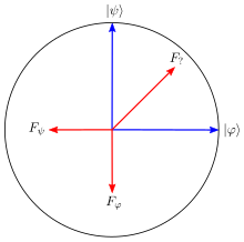
Suppose you have a quantum system with a 2-dimensional Hilbert space that you know is in either the state ${\displaystyle |\psi \rangle }$ or the state ${\displaystyle |\varphi \rangle }$, and you want to determine which one it is. If ${\displaystyle |\psi \rangle }$ and ${\displaystyle |\varphi \rangle }$ are orthogonal, this task is easy: the set ${\displaystyle \{|\psi \rangle \langle \psi |,|\varphi \rangle \langle \varphi |\}}$ will form a PVM, and a projective measurement in this basis will determine the state with certainty. If, however, ${\displaystyle |\psi \rangle }$ and ${\displaystyle |\varphi \rangle }$ are not orthogonal, this task is impossible, in the sense that there is no measurement, either PVM or POVM, that will distinguish them with certainty.^[3]: 87 The impossibility of perfectly discriminating between non-orthogonal states is the basis for quantum information protocols such as quantum cryptography, quantum coin flipping, and quantum money.

The task of unambiguous quantum state discrimination (UQSD) is the next best thing: to never make a mistake about whether the state is ${\displaystyle |\psi \rangle }$ or ${\displaystyle |\varphi \rangle }$, at the cost of sometimes having an inconclusive result. It is possible to do this with projective measurements.^[8] For example, if you measure the PVM ${\displaystyle \{|\psi \rangle \langle \psi |,|\psi ^{\perp }\rangle \langle \psi ^{\perp }|\}}$, where ${\displaystyle |\psi ^{\perp }\rangle }$ is the quantum state orthogonal to ${\displaystyle |\psi \rangle }$, and obtain result ${\displaystyle |\psi ^{\perp }\rangle \langle \psi ^{\perp }|}$, then you know with certainty that the state was ${\displaystyle |\varphi \rangle }$. If the result was ${\displaystyle |\psi \rangle \langle \psi |}$, then it is inconclusive. The analogous reasoning holds for the PVM ${\displaystyle \{|\varphi \rangle \langle \varphi |,|\varphi ^{\perp }\rangle \langle \varphi ^{\perp }|\}}$, where ${\displaystyle |\varphi ^{\perp }\rangle }$ is the state orthogonal to ${\displaystyle |\varphi \rangle }$.

This is unsatisfactory, though, as you can't detect both ${\displaystyle |\psi \rangle }$ and ${\displaystyle |\varphi \rangle }$ with a single measurement, and the probability of getting a conclusive result is smaller than with POVMs. The POVM that gives the highest probability of a conclusive outcome in this task is given by ^[8][9]

${\displaystyle F_{\psi }={\frac {1}{1+|\langle \varphi |\psi \rangle |}}|\varphi ^{\perp }\rangle \langle \varphi ^{\perp }|}$

${\displaystyle F_{\varphi }={\frac {1}{1+|\langle \varphi |\psi \rangle |}}|\psi ^{\perp }\rangle \langle \psi ^{\perp }|}$

${\displaystyle F_{?}=\operatorname {I} -F_{\psi }-F_{\varphi }={\frac {2|\langle \varphi |\psi \rangle |}{1+|\langle \varphi |\psi \rangle |}}|\gamma \rangle \langle \gamma |,}$

where

${\displaystyle |\gamma \rangle ={\frac {1}{\sqrt {2(1+|\langle \varphi |\psi \rangle |)}}}(|\psi \rangle +e^{i\arg(\langle \varphi |\psi \rangle )}|\varphi \rangle ).}$

Note that ${\displaystyle \operatorname {tr} (|\varphi \rangle \langle \varphi |F_{\psi })=\operatorname {tr} (|\psi \rangle \langle \psi |F_{\varphi })=0}$, so when outcome ${\displaystyle \psi }$ is obtained we are certain that the quantum state is ${\displaystyle |\psi \rangle }$, and when outcome ${\displaystyle \varphi }$ is obtained we are certain that the quantum state is ${\displaystyle |\varphi \rangle }$.

The probability of having a conclusive outcome is given by

${\displaystyle 1-|\langle \varphi |\psi \rangle |,}$

when the quantum system is in state ${\displaystyle |\psi \rangle }$ or ${\displaystyle |\varphi \rangle }$ with the same probability. This result is known as the Ivanović-Dieks-Peres limit, named after the authors who pioneered UQSD research.^[10][11][12]

Since the POVMs are rank-1, we can use the simple case of the construction above to obtain a projective measurement that physically realises this POVM. Labelling the three possible states of the enlarged Hilbert space as ${\displaystyle |{\text{result ψ}}\rangle }$, ${\displaystyle |{\text{result φ}}\rangle }$, and ${\displaystyle |{\text{result ?}}\rangle }$, we see that the resulting unitary ${\displaystyle U_{\text{UQSD}}}$ takes the state ${\displaystyle |\psi \rangle }$ to

${\displaystyle U_{\text{UQSD}}|\psi \rangle ={\sqrt {1-|\langle \varphi |\psi \rangle |}}|{\text{result ψ}}\rangle +{\sqrt {|\langle \varphi |\psi \rangle |}}|{\text{result ?}}\rangle ,}$

and similarly it takes the state ${\displaystyle |\varphi \rangle }$ to

${\displaystyle U_{\text{UQSD}}|\varphi \rangle ={\sqrt {1-|\langle \varphi |\psi \rangle |}}|{\text{result φ}}\rangle +e^{-i\arg(\langle \varphi |\psi \rangle )}{\sqrt {|\langle \varphi |\psi \rangle |}}|{\text{result ?}}\rangle .}$

A projective measurement then gives the desired results with the same probabilities as the POVM.

This POVM has been used to experimentally distinguish non-orthogonal polarisation states of a photon. The realisation of the POVM with a projective measurement was slightly different from the one described here.^[13][14]

See also

• SIC-POVM
• Quantum measurement
• Mathematical formulation of quantum mechanics
• Density matrix
• Quantum operation
• Projection-valued measure
• Vector measure

References

• POVMs
  • K. Kraus, States, Effects, and Operations, Lecture Notes in Physics 190, Springer (1983).
  • A.S. Holevo, Probabilistic and statistical aspects of quantum theory, North-Holland Publ. Cy., Amsterdam (1982).

External links

• Interactive demonstration about quantum state discrimination

References

- ^ Peres, Asher; Terno, Daniel R. (2004). "Quantum information and relativity theory". Reviews of Modern Physics. 76 (1): 93–123. arXiv:quant-ph/0212023. Bibcode:2004RvMP...76...93P. doi:10.1103/RevModPhys.76.93. S2CID 7481797.
- ^ Davies, Edward Brian (1976). Quantum Theory of Open Systems. London: Acad. Press. p. 35. ISBN 978-0-12-206150-9.
- ^ a b c M. Nielsen and I. Chuang, Quantum Computation and Quantum Information, Cambridge University Press, (2000)
- ^ I. M. Gelfand and M. A. Neumark, On the embedding of normed rings into the ring of operators in Hilbert space, Rec. Math. [Mat. Sbornik] N.S. 12(54) (1943), 197–213.
- ^ a b A. Peres. Quantum Theory: Concepts and Methods. Kluwer Academic Publishers, 1993.
- ^ J. Preskill, Lecture Notes for Physics: Quantum Information and Computation, Chapter 3, http://theory.caltech.edu/~preskill/ph229/index.html
- ^ J. Watrous. The Theory of Quantum Information. Cambridge University Press, 2018. Chapter 2.3, https://cs.uwaterloo.ca/~watrous/TQI/
- ^ a b J.A. Bergou; U. Herzog; M. Hillery (2004). "Discrimination of Quantum States". In M. Paris; J. Řeháček (eds.). Quantum State Estimation. Springer. pp. 417–465. doi:10.1007/978-3-540-44481-7_11. ISBN 978-3-540-44481-7.
- ^ Chefles, Anthony (2000). "Quantum state discrimination". Contemporary Physics. 41 (6). Informa UK Limited: 401–424. arXiv:quant-ph/0010114v1. Bibcode:2000ConPh..41..401C. doi:10.1080/00107510010002599. ISSN 0010-7514. S2CID 119340381.
- ^ Ivanovic, I.D. (1987). "How to differentiate between non-orthogonal states". Physics Letters A. 123 (6). Elsevier BV: 257–259. Bibcode:1987PhLA..123..257I. doi:10.1016/0375-9601(87)90222-2. ISSN 0375-9601.
- ^ Dieks, D. (1988). "Overlap and distinguishability of quantum states". Physics Letters A. 126 (5–6). Elsevier BV: 303–306. Bibcode:1988PhLA..126..303D. doi:10.1016/0375-9601(88)90840-7. ISSN 0375-9601.
- ^ Peres, Asher (1988). "How to differentiate between non-orthogonal states". Physics Letters A. 128 (1–2). Elsevier BV: 19. Bibcode:1988PhLA..128...19P. doi:10.1016/0375-9601(88)91034-1. ISSN 0375-9601.
- ^ B. Huttner; A. Muller; J. D. Gautier; H. Zbinden; N. Gisin (1996). "Unambiguous quantum measurement of nonorthogonal states". Physical Review A. 54 (5). APS: 3783–3789. Bibcode:1996PhRvA..54.3783H. doi:10.1103/PhysRevA.54.3783. PMID 9913923.
- ^ R. B. M. Clarke; A. Chefles; S. M. Barnett; E. Riis (2001). "Experimental demonstration of optimal unambiguous state discrimination". Physical Review A. 63 (4). APS: 040305(R). arXiv:quant-ph/0007063. Bibcode:2001PhRvA..63d0305C. doi:10.1103/PhysRevA.63.040305. S2CID 39481893.